Code
from dataclasses import dataclass
import numpy as np
import matplotlib.pyplot as plt
import tensorflow as tf
from skimage import io
from scipy.ndimage import label
from collections import defaultdictDeep learning algorithms need large training datasets to reach high accuracy predictions. This is problematic in the medical domain for which the cost of data collection is high and data from rare conditions is scarce. Current solutions include the generation of synthetic data for rare conditions; however, the synthetic data is a source of over-fitting of the neural network during training because of the lack of diversity of the synthetic images.
Here I will show:
from dataclasses import dataclass
import numpy as np
import matplotlib.pyplot as plt
import tensorflow as tf
from skimage import io
from scipy.ndimage import label
from collections import defaultdict@dataclass
class Param:
train_img_file: str
train_msk_file: str
test_img_file: str
test_msk_file: str
seed: int
crop_size: int
img_size: int
batch: int
lr: float
alpha: float
epochs: int
steps_per_epoch: int
param = Param(
train_img_file="E:/Data/EM3DSEG/training.tif",
train_msk_file="E:/Data/EM3DSEG/training_groundtruth.tif",
test_img_file="E:/Data/EM3DSEG/testing.tif",
test_msk_file="E:/Data/EM3DSEG/testing_groundtruth.tif",
seed=42,
crop_size=320,
img_size=128,
batch=64,
lr=5e-4,
alpha=0.4,
epochs=20,
steps_per_epoch=1000,
)The Electron Microscopy 3D dataset was downloaded from kaggle. It is a multi-tif image stored in param.train_img_file with its ground-truth mitochondria segmentation in param.train_msk_file.
The shape of the training dataset is: (165, 768, 1024)
and the shape of the testing dataset is: (165, 768, 1024)def crop(img, msk):
stacked_img_msk = tf.stack([img,msk], axis=0)
cropped_img_msk = tf.image.random_crop(stacked_img_msk,
size=[2, param.crop_size, param.crop_size, 1],
seed=param.seed)
crop_img = tf.image.resize(cropped_img_msk[0], [param.img_size, param.img_size],
method=tf.image.ResizeMethod.NEAREST_NEIGHBOR)
norm_img = (tf.cast(crop_img, dtype=tf.float32) / 127.5) - 1
crop_msk = tf.image.resize(cropped_img_msk[1], [param.img_size, param.img_size],
method=tf.image.ResizeMethod.NEAREST_NEIGHBOR)
norm_msk = tf.cast(crop_msk, dtype=tf.float32) / 255.
return norm_img, norm_msk# Reading the original multi-tif file with the skimage.io library
# and converting it into tensors
img_ds = tf.data.Dataset.from_tensor_slices(io.imread(param.train_img_file)[...,None])
msk_ds = tf.data.Dataset.from_tensor_slices(io.imread(param.train_msk_file)[...,None])
# Here I am using a random crop function applied on images and masks
ds = tf.data.Dataset.zip((img_ds, msk_ds))
ds = ds.map(crop, num_parallel_calls=tf.data.AUTOTUNE)
ds = ds.shuffle(param.batch*8).batch(param.batch, drop_remainder=True).repeat()
ds = ds.cache().prefetch(buffer_size=tf.data.AUTOTUNE)
# Defining the validation dataset
val_img_ds = tf.data.Dataset.from_tensor_slices(io.imread(param.test_img_file)[...,None])
val_msk_ds = tf.data.Dataset.from_tensor_slices(io.imread(param.test_msk_file)[...,None])
val_ds = tf.data.Dataset.zip((val_img_ds, val_msk_ds))
val_ds = val_ds.map(crop, num_parallel_calls=tf.data.AUTOTUNE)
val_ds = val_ds.shuffle(param.batch*8).batch(param.batch, drop_remainder=True)
val_ds = val_ds.cache().prefetch(buffer_size=tf.data.AUTOTUNE)Visualizing an image batch with the mitochondria ground-truth segmentation as contours:
f, ax = plt.subplots(3,3, figsize=(8,8))
for imgs, msks in ds.take(1):
    for i, a in enumerate(ax.flatten()):
        a.imshow(imgs[i], cmap='gray')
        if msks[i].numpy().sum() > 0:
            a.contour(msks[i,:,:,0])
        a.axis('off')
plt.show()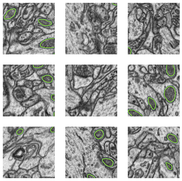
I am using the Pix2Pix architecture for the generator network and a PatchGAN dicriminator from (Isola et al. 2017).
def l1_loss(y_true, y_pred):
    return tf.reduce_sum(tf.abs(tf.cast(y_pred, tf.float32) - tf.cast(y_true, tf.float32)), axis=-1)

class GAN:
    def __init__(self, in_channels=1, out_channels=1):
        self.img_size = param.img_size
        self.output_channels = out_channels
        self.input_channels = in_channels

    def conv_layer_discriminator(self, x, filters, name, init_kernel, strides=2, bn=True):
        x = tf.keras.layers.Conv2D(filters, 4, strides=strides, padding='same', kernel_initializer=init_kernel, name=name + '_conv')(x)
        if bn:
            x = tf.keras.layers.BatchNormalization(name=name + '_bn')(x)
        return tf.keras.layers.LeakyReLU(0.2, name=name + '_lrelu')(x)

    def build_discriminator(self):
        init_kernel = tf.keras.initializers.RandomNormal(stddev=0.02)
        vol = tf.keras.Input(shape=(self.img_size, self.img_size, self.output_channels), name="volume")
        seg = tf.keras.Input(shape=(self.img_size, self.img_size, self.input_channels), name="segmentation")
        x = tf.keras.layers.Concatenate()([seg, vol])
        for i, f in enumerate([64, 128, 256, 512, 512]):
            bn = False if i == 0 else True
            s = 1 if i == 4 else 2
            x = self.conv_layer_discriminator(x, f, f"C{f}_s{s}", init_kernel, strides=s, bn=bn)
        # Patch output
        x = tf.keras.layers.Conv2D(1, (4, 4), padding="same", kernel_initializer=init_kernel)(x)
        # patch_out = tf.keras.layers.Activation("sigmoid")(x)
        model = tf.keras.Model([seg, vol], x)

        return model

    def encoder_layer_generator(self, filters, name, init_kernel, bn=True):
        result = tf.keras.Sequential(name=name)
        result.add(tf.keras.layers.Conv2D(filters, 3, strides=2, padding='same', kernel_initializer=init_kernel, name=name + '_conv'))
        if bn:
            result.add(tf.keras.layers.BatchNormalization(name=name + '_bn'))
        result.add(tf.keras.layers.LeakyReLU(0.2, name=name + '_lrelu'))
        return result

    def decoder_layer_generator(self, filters, name, init_kernel, do=False):
        result = tf.keras.Sequential(name=name)
        result.add(tf.keras.layers.Conv2DTranspose(filters, 4, strides=2, padding='same', kernel_initializer=init_kernel,
                                   name=name + '_deconv'))
        result.add(tf.keras.layers.BatchNormalization(name=name + '_bn'))
        if do:
            result.add(tf.keras.layers.Dropout(0.5, name=name + '_do'))
        result.add(tf.keras.layers.Activation('relu', name=name + '_relu'))
        return result

    def up_decoder_layer_generator(self, filters, name, init_kernel, do=False):
        result = tf.keras.Sequential(name=name)
        result.add(tf.keras.layers.UpSampling2D(size=(2, 2), name=name + '_upsample'))
        result.add(tf.keras.layers.Conv2D(filters, 3, padding='same', kernel_initializer=init_kernel, name=name + '_conv'))
        result.add(tf.keras.layers.BatchNormalization(name=name + '_bn'))
        if do:
            result.add(tf.keras.layers.Dropout(0.5, name=name + '_do'))
        result.add(tf.keras.layers.Activation('relu', name=name + '_relu'))
        return result

    def build_generator(self, upsample=False):
        init_kernel = tf.keras.initializers.RandomNormal(stddev=0.02)
        seg_in = tf.keras.Input(shape=(self.img_size, self.img_size, self.input_channels), name='seg')
        down_stack, up_stack = [], []
        for i, f in enumerate([64, 128, 256, 512, 512, 512, 512]):
            bn = False if i == 0 else True
            down_stack.append(self.encoder_layer_generator(f, f"E{f}_{i + 1}", init_kernel, bn=bn))
        for i, f in enumerate([512, 512, 512, 256, 128, 64]):
            do = True if i <= 2 else False
            if upsample:
                up_stack.append(self.up_decoder_layer_generator(f, f"D{f}_{i + 1}", init_kernel, do=do))
            else:
                up_stack.append(self.decoder_layer_generator(f, f"D{f}_{i + 1}", init_kernel, do=do))
        x = seg_in
        skips = []
        for down in down_stack:
            x = down(x)
            skips.append(x)
        skips = reversed(skips[:-1])
        for up, skip in zip(up_stack, skips):
            x = up(x)
            x = tf.keras.layers.Concatenate()([x, skip])
        if upsample:
            x = tf.keras.layers.UpSampling2D(size=(2, 2), name='last_up')(x)
            x = tf.keras.layers.Conv2D(1, (3, 3), name='last_conv', padding='same')(x)
        else:
            x = tf.keras.layers.Conv2DTranspose(1, 4, strides=2, padding='same', kernel_initializer=init_kernel, name='last')(x)
        x = tf.keras.layers.Activation('tanh')(x)
        return tf.keras.Model(seg_in, x)

    def compile_dis_gen_gan(self, lr=1e-3, upsample=False):
        dis = self.build_discriminator()
        dis.trainable = False
        gen = self.build_generator(upsample)
        seg = tf.keras.Input(shape=(self.img_size, self.img_size, self.input_channels))
        gen_out = gen(seg)
        dis_out = dis([seg, gen_out])
        gan = tf.keras.Model(seg, [dis_out, gen_out])
        gan.compile(optimizer=tf.keras.Adam(learning_rate=lr, beta_1=0.9, beta_2=0.999, epsilon=1e-08),
                    loss=['binary_crossentropy', l1_loss], loss_weights=[1, 100])
        dis.trainable = True
        dis.compile(optimizer=tf.keras.Adam(learning_rate=lr*1e-3, beta_1=0.9, beta_2=0.999, epsilon=1e-08), loss='binary_crossentropy')
        return dis, gen, gan
# Models
gan_model = GAN()
discriminator = gan_model.build_discriminator()
generator = gan_model.build_generator()
# Optmizers
dis_opt = tf.keras.optimizers.Adam(learning_rate=param.lr * 1e-3,
beta_1=0.9, beta_2=0.999, epsilon=1e-08)
gen_opt = tf.keras.optimizers.Adam(learning_rate=param.lr,
beta_1=0.9, beta_2=0.999, epsilon=1e-08)
# Loss function
loss_fn = tf.keras.losses.BinaryCrossentropy(from_logits=True)
# Discriminator targets
n_patches = discriminator.output_shape[1]
y_real = tf.ones(shape=(param.batch, n_patches, n_patches, 1))
y_fake = tf.zeros_like(y_real)# Training
epochs = 50
steps_per_epochs = param.steps_per_epoch
for e in range(epochs):
for imgs, msks in ds.take(steps_per_epochs):
fake_img = generator(msks, training=False)
# Discriminator training on false images
with tf.GradientTape() as tape:
false_preds = discriminator([msks, fake_img], training=True)
d_fake_loss = loss_fn(y_fake, false_preds)
d_fake_grad = tape.gradient(d_fake_loss, discriminator.trainable_variables)
dis_opt.apply_gradients(zip(d_fake_grad, discriminator.trainable_variables))
# Discriminator training on true images
with tf.GradientTape() as tape:
true_preds = discriminator([msks, imgs], training=True)
d_real_loss = loss_fn(y_real, true_preds)
d_real_grad = tape.gradient(d_real_loss, discriminator.trainable_variables)
dis_opt.apply_gradients(zip(d_real_grad, discriminator.trainable_variables))
# Generator training
with tf.GradientTape() as tape:
gan_img = generator(msks, training=True)
gan_preds = discriminator([msks, gan_img], training=False)
g_mean_loss = loss_fn(y_real, gan_preds) + 100 * l1_loss(imgs, gan_img)
gan_grad = tape.gradient(g_mean_loss, generator.trainable_variables)
gen_opt.apply_gradients(zip(gan_grad, generator.trainable_variables))The trained generator can produce synthetic images from the input masks. We can observe a checkerboard artifact produced by the decoder branch that use a transposed convolution layer (the trainable Conv2DTranspose).
f, ax = plt.subplots(3,3, figsize=(8,8))
for imgs, msks in ds.take(1):
    gan_imgs = generator(msks)
    for i, a in enumerate(ax.flatten()):
        a.imshow(gan_imgs[i], cmap='gray')
        if msks[i].numpy().sum() > 0:
            a.contour(msks[i,:,:,0])
        a.axis('off')
plt.show()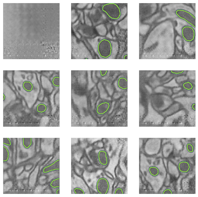
State-of-the art semantic segmentation networks includes variations of the U-net architure defined by (Ronneberger, Fischer, and Brox 2015). I am using a lightweight variation defined by (Chaudhary et al. 2019) called RITnet. They used the convolution block of the DenseNet model (Huang et al. 2016) into the U-net architecture to reduce the number of parameters. This network is particularly well suited to small medical datasets because of the extensive use of Dropout layers to fight over-fitting.
class RITnet():
    def __init__(self, channels=32, img_size=param.img_size, num_classes=1):
        self.img_size = img_size
        self.ch = channels
        self.num_classes = num_classes
        super(RITnet).__init__()

    def _conv_2x(self):
        x = tf.keras.Sequential()
        x.add(tf.keras.layers.Conv2D(self.ch, kernel_size=1, padding="valid"))
        x.add(tf.keras.layers.Conv2D(self.ch, kernel_size=3, padding="same"))
        x.add(tf.keras.layers.Dropout(0.5))
        x.add(tf.keras.layers.LeakyReLU())
        return x

    def _conv_1x(self):
        x = tf.keras.Sequential()
        x.add(tf.keras.layers.Conv2D(self.ch, kernel_size=3, padding="same"))
        x.add(tf.keras.layers.Dropout(0.5))
        x.add(tf.keras.layers.LeakyReLU())
        return x

    def down_block(self, inputs):
        x = tf.keras.layers.AveragePooling2D((2,2))(inputs)
        x1 = self._conv_1x()(x)
        x2 = tf.keras.layers.Concatenate()([x1, x])
        x = self._conv_2x()(x2)
        x = tf.keras.layers.Concatenate()([x2, x])
        x = self._conv_2x()(x)
        return tf.keras.layers.BatchNormalization()(x)

    def up_block(self, inputs, skip):
        x = tf.keras.layers.UpSampling2D((2,2))(inputs)
        x = tf.keras.layers.Concatenate()([skip, x])
        x1 = self._conv_2x()(x)
        x = tf.keras.layers.Concatenate()([x1,x])
        x = self._conv_2x()(x)
        return x

    def generate(self):
        inputs = tf.keras.Input(shape=(self.img_size, self.img_size, 1))
        x = inputs
        x1 = self.down_block(x)
        x2 = self.down_block(x1)
        x3 = self.down_block(x2)
        x4 = self.down_block(x3)
        x5 = self.down_block(x4)
        x6 = self.up_block(x5, x4)
        x7 = self.up_block(x6, x3)
        x8 = self.up_block(x7, x2)
        x9 = self.up_block(x8, x1)
        x10 = tf.keras.layers.UpSampling2D((2,2))(x9)
        x11 = tf.keras.layers.Conv2D(self.num_classes, kernel_size=1, padding="valid")(x10)
        return tf.keras.Model(inputs, x11)

# Evaluation function
def dice_LiTS(reference, prediction, smooth=1e-6, threshold=0.5):
    prediction = tf.math.greater(prediction, threshold)
    prediction = tf.cast(prediction, tf.bool)
    reference = tf.cast(reference, tf.bool)
    intersect = tf.math.count_nonzero(prediction & reference, dtype=tf.dtypes.float64)
    size_i1 = tf.math.count_nonzero(prediction, dtype=tf.dtypes.float64)
    size_i2 = tf.math.count_nonzero(reference, dtype=tf.dtypes.float64)
    return (2. * intersect + smooth) / (size_i1 + size_i2 + smooth)

def plot_history(history):
    f, ax = plt.subplots(1,2, figsize=(10,4))
    ax[0].plot(history['epoch'], history['train_loss'], color='tab:red', label='training')
    ax[0].plot(history['epoch'], history['val_loss'], color='tab:blue', label='validation')
    ax[0].set_ylabel('loss')
    ax[0].set_xlabel('epoch')
    ax[0].legend()
    ax[1].plot(history['epoch'], history['train_dice'], color='tab:red')
    ax[1].plot(history['epoch'], history['val_dice'], color='tab:blue')
    ax[1].set_ylabel('dice')
    ax[1].set_xlabel('epoch')
    plt.show()
ritnet = RITnet()
seg_model = ritnet.generate()Model training:
epochs=param.epochs
steps_per_epoch=param.steps_per_epoch
loss_fn = tf.keras.losses.BinaryCrossentropy(from_logits=True)
act_fn = tf.math.sigmoid
opt = tf.keras.optimizers.Adam(learning_rate=param.lr)
history = defaultdict(list)
metrics = {'train_loss': tf.keras.metrics.Mean(), 'train_dice': tf.keras.metrics.Mean(),
          'val_loss': tf.keras.metrics.Mean(), 'val_dice': tf.keras.metrics.Mean()}

for e in range(epochs):
    # Reset logger
    for k,v in metrics.items():
        v.reset_states()
    history['epoch'].append(e)
    # Train
    for img, msk in ds.take(steps_per_epoch):
        with tf.GradientTape() as tape:
            logits = seg_model(img, training=True)
            loss = loss_fn(msk, logits)
        grads = tape.gradient(loss, seg_model.trainable_variables)
        opt.apply_gradients(zip(grads, seg_model.trainable_variables))
        # Logging
        metrics['train_loss'].update_state(loss)
        metrics['train_dice'].update_state(dice_LiTS(msk, act_fn(logits)))

    # Validation
    for val_img,val_msk in val_ds:
        val_logits = seg_model(val_img, training=False)
        val_loss = loss_fn(val_msk, val_logits)
        metrics['val_loss'].update_state(val_loss)
        metrics['val_dice'].update_state(dice_LiTS(val_msk, act_fn(val_logits)))

    # logging
    history['train_loss'].append(metrics['train_loss'].result())
    history['train_dice'].append(metrics['train_dice'].result())
    history['val_loss'].append(metrics['val_loss'].result())
    history['val_dice'].append(metrics['val_dice'].result())

    print(f"epoch: {e:3d} loss: {history['train_loss'][-1]:.3f} dice: {history['train_dice'][-1]:.3f} val_loss: {history['val_loss'][-1]:.3f} val_dice: {history['val_dice'][-1]:.3f}")
plot_history(history)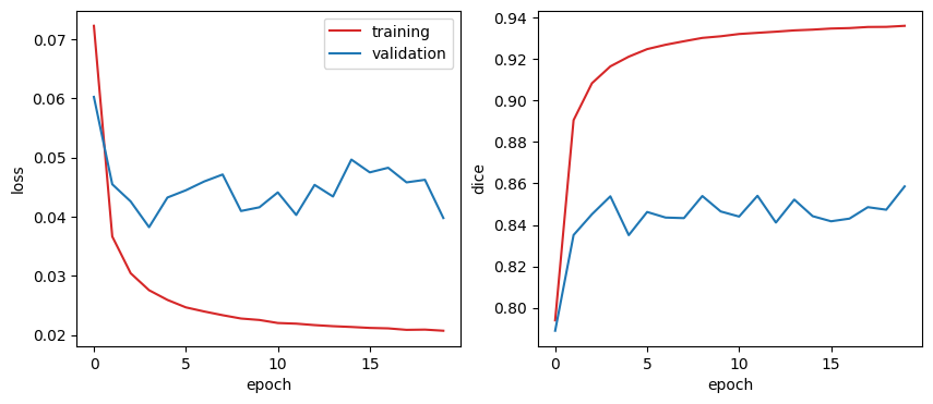
We can observe a characteristic over-fitting pattern of the training curves compared to the validation curves. The training loss become significantly lower than the validation loss around epoch 5 and the validation dice could not match the training dice already at the training onset. The over-fitting can be mitigated by using data augmentation and / or additional training data.
Instead of using the training dataset to train the segmentaion model, we use the synthetic images produced by the trained generator of the GAN.
ritnet = RITnet()
synth_seg_model = ritnet.generate()epochs=param.epochs
steps_per_epoch=param.steps_per_epoch
history = defaultdict(list)
metrics = {'train_loss': tf.keras.metrics.Mean(), 'train_dice': tf.keras.metrics.Mean(),
'val_loss': tf.keras.metrics.Mean(), 'val_dice': tf.keras.metrics.Mean()}
for e in range(epochs):
# Reset logger
for k,v in metrics.items():
v.reset_states()
history['epoch'].append(e)
# Train
for img, msk in ds.take(steps_per_epoch):
gan_img = generator(msk)
with tf.GradientTape() as tape:
logits = synth_seg_model(gan_img, training=True)
loss = loss_fn(msk, logits)
grads = tape.gradient(loss, synth_seg_model.trainable_variables)
opt.apply_gradients(zip(grads, synth_seg_model.trainable_variables))
# Logging
metrics['train_loss'].update_state(loss)
metrics['train_dice'].update_state(dice_LiTS(msk, act_fn(logits)))
# Validation
for val_img,val_msk in val_ds:
val_logits = synth_seg_model(val_img, training=False)
val_loss = loss_fn(val_msk, val_logits)
metrics['val_loss'].update_state(val_loss)
metrics['val_dice'].update_state(dice_LiTS(val_msk, act_fn(val_logits)))
# logging
history['train_loss'].append(metrics['train_loss'].result())
history['train_dice'].append(metrics['train_dice'].result())
history['val_loss'].append(metrics['val_loss'].result())
history['val_dice'].append(metrics['val_dice'].result())
print(f"epoch: {e:3d} loss: {history['train_loss'][-1]:.3f} dice: {history['train_dice'][-1]:.3f} val_loss: {history['val_loss'][-1]:.3f} val_dice: {history['val_dice'][-1]:.3f}")plot_history(history)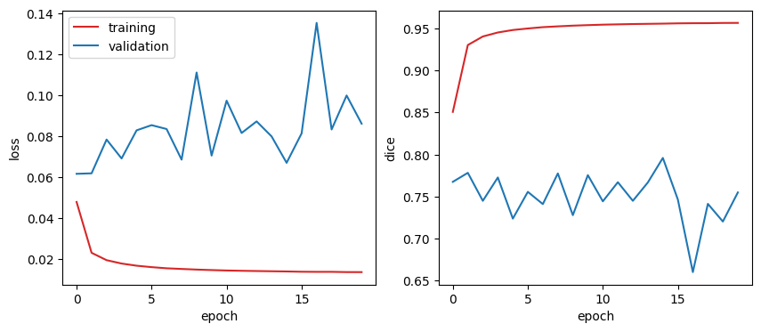
We can observe that the over-fitting problem is worst when using the synthetic data compared to the original training data. This may be explained by:
I investigated the data quality problem and find no correlation between the quality of the generated synthetic images, mesured by the Frechet Inception Distance, and the evaluation dice of the trained segmentation network. This led me to investigate the data augmentation effect of the synthetic data on the segmentation training.
Instead of the original segmentation masks as generator input we can use artificial segmetation masks to increase the diversity of the produced synthetic images.
def compose_mask(msk):
    comp_msks = np.zeros_like(msk.numpy())
    for i,m in enumerate(msk.numpy()):
        comp_msk = np.zeros_like(m)
        lab, n_feats = label(m)
        x = np.random.randint(3, n_feats) if n_feats > 3 else n_feats
        comp_samples = np.random.choice(np.arange(1, 1+n_feats), size=x)
        for c in comp_samples:
            single_component = lab == c
            single_component = np.rot90(single_component, k=np.random.randint(1,4))
            single_component = np.flip(single_component, axis=np.random.randint(0,1))
            comp_msk = np.where(single_component, single_component, comp_msk)
        comp_msks[i] = comp_msk
    return comp_msks

def rescale_img(img):
    """
    Normalize image values into the [0,1] range
    :param img:
    :return: img
    """
    min_img = np.min(img)
    max_img = np.max(img)
return (img - min_img) / (max_img - min_img)f, ax = plt.subplots(2,6, figsize=(12,4), sharex=True, sharey=True)
for img, msk in ds.take(1):
comp_msks = compose_mask(msk)
syn_imgs = generator(comp_msks)
for i, (m, c, s) in enumerate(zip(msk[:6], comp_msks[:6], syn_imgs[:6])):
ax[0,i].imshow(img[i], cmap='gray')
ax[0,i].contour(m[:,:,0])
ax[1,i].imshow(s, cmap='gray')
ax[1,i].contour(c[:,:,0])
ax[0,0].set_ylabel('Original')
ax[1,0].set_ylabel('Synthetic')
plt.show()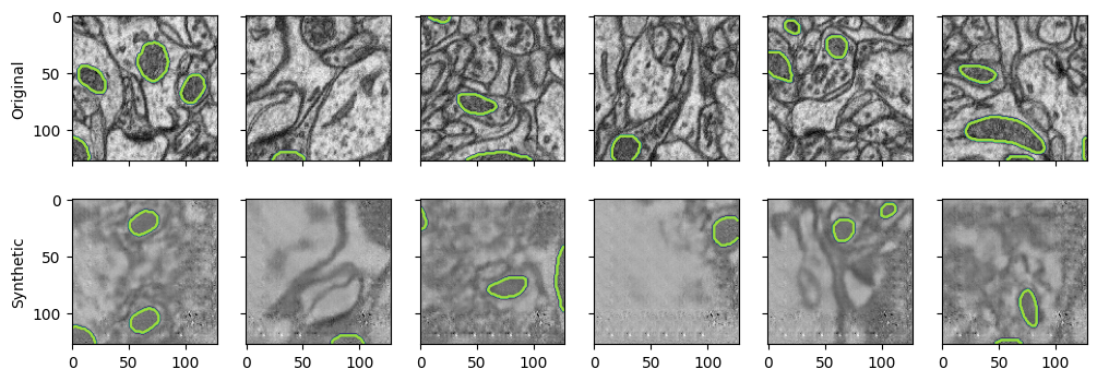
ritnet = RITnet()
artsynth_seg_model = ritnet.generate()
gan_model = GAN()
discriminator = gan_model.build_discriminator()
generator = gan_model.build_generator()

# Optmizers
dis_opt = tf.keras.optimizers.Adam(learning_rate=param.lr * 1e-3, beta_1=0.9, beta_2=0.999, epsilon=1e-08)
gen_opt = tf.keras.optimizers.Adam(learning_rate=param.lr, beta_1=0.9, beta_2=0.999, epsilon=1e-08)
opt = tf.keras.optimizers.Adam(learning_rate=param.lr)

# Loss function
sup_loss_fn = tf.keras.losses.BinaryCrossentropy(from_logits=False)
gan_loss_fn = tf.keras.losses.BinaryCrossentropy(from_logits=True)

# Activation function
act_fn = tf.math.sigmoid

# Discriminator targets
n_patches = discriminator.output_shape[1]
y_real = tf.ones(shape=(param.batch, n_patches, n_patches, 1))
y_fake = tf.zeros_like(y_real)epochs=param.epochs
steps_per_epoch=param.steps_per_epoch
history = defaultdict(list)
metrics = {'train_loss': tf.keras.metrics.Mean(), 'train_dice': tf.keras.metrics.Mean(),
'val_loss': tf.keras.metrics.Mean(), 'val_dice': tf.keras.metrics.Mean()}
for e in range(epochs):
loss_ratio = param.alpha * np.log(e + 1)
# Reset logger
for k,v in metrics.items():
v.reset_states()
history['epoch'].append(e)
# Train
for img, msk in ds.take(steps_per_epoch):
# GAN training
fake_img = generator(msk, training=False)
# Discriminator training on false images
with tf.GradientTape() as tape:
false_preds = discriminator([msk, fake_img], training=True)
d_fake_loss = gan_loss_fn(y_fake, false_preds)
d_fake_grad = tape.gradient(d_fake_loss, discriminator.trainable_variables)
dis_opt.apply_gradients(zip(d_fake_grad, discriminator.trainable_variables))
# Discriminator training on true images
with tf.GradientTape() as tape:
true_preds = discriminator([msk, img], training=True)
d_real_loss = gan_loss_fn(y_real, true_preds)
d_real_grad = tape.gradient(d_real_loss, discriminator.trainable_variables)
dis_opt.apply_gradients(zip(d_real_grad, discriminator.trainable_variables))
# Generator training
with tf.GradientTape() as tape:
gan_img = generator(msk, training=True)
gan_preds = discriminator([msk, gan_img], training=False)
g_mean_loss = gan_loss_fn(y_real, gan_preds) + 100 * l1_loss(img, gan_img)
gan_grad = tape.gradient(g_mean_loss, generator.trainable_variables)
gen_opt.apply_gradients(zip(gan_grad, generator.trainable_variables))
# RITnet training
comp_msks = compose_mask(msk)
gan_img = generator(comp_msks, training=False)
# Score generator image
dis_pred = discriminator([msk, gan_img], training=False)
isreal_score = 1 - np.clip(sup_loss_fn(y_real, act_fn(dis_pred)), 0, 1)
with tf.GradientTape() as tape:
logits = artsynth_seg_model(img, training=True)
pred = act_fn(logits)
pred_loss = sup_loss_fn(msk, pred)
syn_logits = artsynth_seg_model(gan_img, training=True)
syn_pred = act_fn(syn_logits)
syn_loss = sup_loss_fn(comp_msks, syn_pred)
loss = pred_loss + loss_ratio * syn_loss * isreal_score
grads = tape.gradient(loss, artsynth_seg_model.trainable_variables)
opt.apply_gradients(zip(grads, artsynth_seg_model.trainable_variables))
# Logging
metrics['train_loss'].update_state(loss)
metrics['train_dice'].update_state(dice_LiTS(msk, pred))
# Validation
for val_img,val_msk in val_ds:
val_logits = artsynth_seg_model(val_img, training=False)
val_loss = loss_fn(val_msk, val_logits)
metrics['val_loss'].update_state(val_loss)
metrics['val_dice'].update_state(dice_LiTS(val_msk, act_fn(val_logits)))
# logging
history['train_loss'].append(metrics['train_loss'].result())
history['train_dice'].append(metrics['train_dice'].result())
history['val_loss'].append(metrics['val_loss'].result())
history['val_dice'].append(metrics['val_dice'].result())
print(f"epoch: {e:3d} loss: {history['train_loss'][-1]:.3f} dice: {history['train_dice'][-1]:.3f} val_loss: {history['val_loss'][-1]:.3f} val_dice: {history['val_dice'][-1]:.3f}")plot_history(history)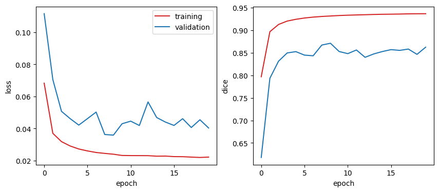
The integration of the training on the synthetic dataset during the supervised training was made using the following loss formula: \[ loss = BCE(y, \mathscr{M}(x)) + \alpha \times BCE(s, \hat{s}) \times (1 - BCE(\mathbb{1}, \mathscr{D}(s, \mathscr{G}(s)))) \] \(\mathscr{M}, \mathscr{D}, \mathscr{G}\) are the segmentation, discriminator and generator models, respectively. The synhtetic image and mask batches are represented by \(\hat{s}\) and \(s\). \(\mathbb{1}\) represents the matix of ones of the same size as the discriminator output. The binary crossentropy formula is : \[ BCE(Y,\hat{Y}) = -\frac{1}{N}\sum_{i=0}^{N}(y_i \times log(\hat{y_i}) + (1 - y_i) \times log(1 - \hat{y_i}))\] and \[ \alpha = SLR \times log(t + 1)\] is the progressive synthetic loss ratio (SLR).
The progressive introduction of the synthetic loss during training and the scoring of generated images by the discriminator protect the training of the segmentation network from unrealistic images. The synthetic dataset is a good regularizer of training.

This work is licensed under a Creative Commons Attribution-ShareAlike 4.0 International License.